Softmax Regression ｜ Softmax 回归

Softmax 定义 #

Softmax 回归虽然名字叫回归，单实际上以一个分类模型。回归是估计一个连续值，对于神经网络来说，它的输出是一个神经元，而分类是预测一个离散的类别，输出是一组向量，这组向量只有一个项是 1，其余项都为 0. 下面是 softmax 函数的定义 $$ \hat{\mathbf{y}} = softmax(\mathbf{o}) $$ ，其中 o 表示输出的一组向量，oi 就是其中一个表示概率的分类。这里的 softmax 表示对输出的向量进行施加一个 softmax 作用，具体的操作如下 $$ \begin{align*} \hat{\mathbf{y}}_i = \frac{e^{o_i}}{\sum {e^{o_k}}} \end{align*} $$ 这里的意思是对于最终估计项 yi 来说，它的值可以通过对第 i 项的输出 oi 做指数运算，再除以输出项每一项做指数运算的和。因为做了指数化，所以保证每一项都是非负的。

softmax 衡量预测精度的损失函数采用交叉熵损失函数，它的定义如下 $$ L(\mathbf{y}, \hat{\mathbf{y}}) = -\sum_{k=1}^K y_k \log \hat{y}_k = -ylog\hat{y}_y $$ ，因为真实的标签中只有一项是 1，所以它就是真实项预测值的概率，这一项的概率越大，值越接近于 0。

它的梯度是真实概率和预测概率的区别，下面是关于梯度的推导， $$ l(\mathbf{y}, \hat{\mathbf{y}}) = - \sum_i y_i \log \hat{y}_i $$

$$ = - \sum_i y_i \log \left( \frac{\exp(o_i)}{\sum_j \exp(o_j)} \right) $$

$$ = - \sum_i y_i \left( o_i - \log \left( \sum_j \exp(o_j) \right) \right) $$

$$ = - \sum_i y_i o_i + \sum_i y_i \log \left( \sum_j \exp(o_j) \right) $$

$$ = - \sum_i y_i o_i + \log \left( \sum_j \exp(o_j) \right) $$

$$ \frac{\partial J}{\partial \mathbf{o}_i} = -y_i + \left( \frac{\exp(o_i)}{\sum_j \exp(o_j)} \right) = softmax(\mathbf{o_i}) - y_i $$

softmax的从零开始实现 #

在开始之前我们首先需要导入一些依赖的库

%matplotlib inline
import torch
import torchvision
from torch.utils import data
from torchvision import transforms
from matplotlib import pyplot as plt
from IPython import display
from matplotlib_inline import backend_inline
backend_inline.set_matplotlib_formats('svg')

数据集采用公开数据集 FashionMNIST，它是一堆物体的图像数据集，如下图所示，

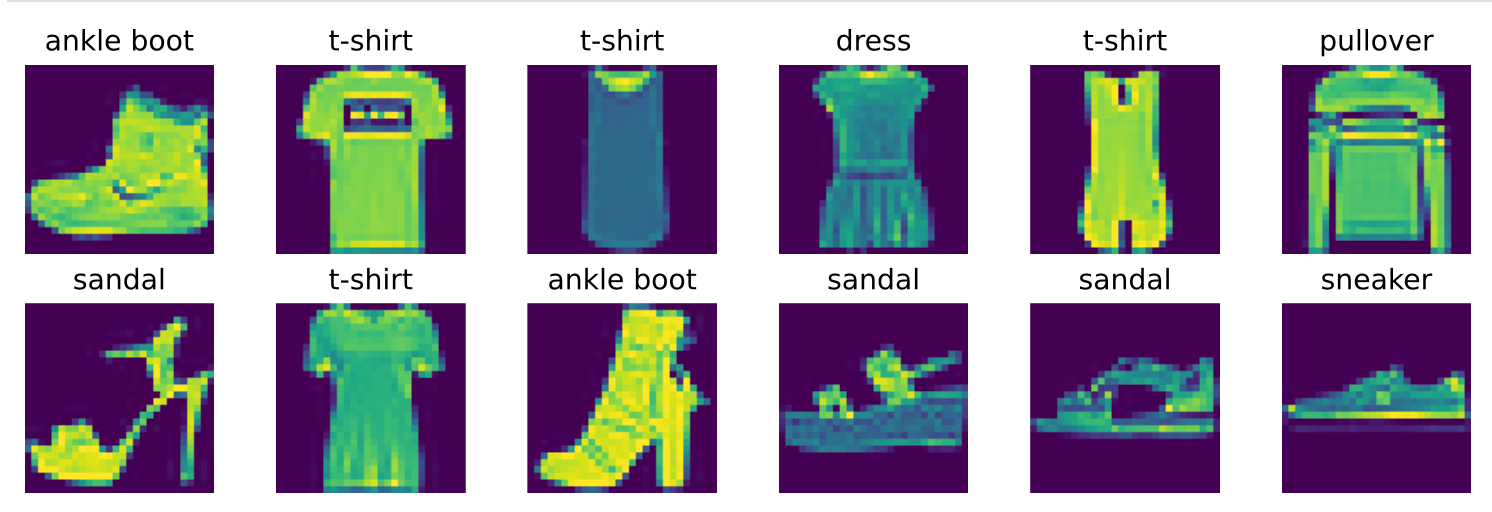
这个数据集一共有十类标签，都是和衣服相关的数据。其中每张图片是 (1，28，28) 的规格，都是黑白的图片。上面显示的图片中有颜色是因为我使用 matplotlib 的 imshow 函数显示时，默认会使用一个颜色映射（colormap）来将灰度值映射为彩色。

然后定义一个读取数据的函数，batch_size 表示一批的个数，resize 可以使得图片变得更大。数据本身是放在 pytorch 官网的，可以直接通过官方提供的 api 下载下来，

def load_data_fashion_mnist(batch_size, resize=None):  
    """下载Fashion-MNIST数据集，然后将其加载到内存中。"""
    trans = [transforms.ToTensor()]
    if resize:
        trans.insert(0, transforms.Resize(resize))
    trans = transforms.Compose(trans)
    mnist_train = torchvision.datasets.FashionMNIST(root="../data",
                                                    train=True,
                                                    transform=trans,
                                                    download=True)
    mnist_test = torchvision.datasets.FashionMNIST(root="../data",
                                                   train=False,
                                                   transform=trans,
                                                   download=True)
    return (data.DataLoader(mnist_train, batch_size, shuffle=True,
                            num_workers=4),
            data.DataLoader(mnist_test, batch_size, shuffle=False,
                            num_workers=4))

下一步定义模型和损失函数。首先定义输入的维度是 784，视为28*28=784的向量，需要把原来的三维图像数据拉平。这里忽略拉平之后可能会造成空间上信息的损耗。由于数据集有10个类别，所以网络输出维度是10。其余函数的实现都和模型定义一致。

num_inputs = 784
num_outputs = 10

W = torch.normal(0, 0.01, size=(num_inputs, num_outputs), requires_grad=True)
b = torch.zeros(num_outputs, requires_grad=True)

def softmax(X):
    X_exp = torch.exp(X)
    partition = X_exp.sum(1, keepdim=True)
    return X_exp / partition

X = torch.normal(0, 1, (2, 5))
X_prob = softmax(X)
X_prob, X_prob.sum(1)

def net(X):
    return softmax(torch.matmul(X.reshape((-1, W.shape[0])), W) + b)

def cross_entropy(y_hat, y):
    return -torch.log(y_hat[range(len(y_hat)), y])

再定义预测模型精度的函数，accuracy 函数是对估计的 y 和实际的 y 进行比较。因为真实的 y 是一组向量，有多少个 y 就应该有多少个带标签的 y_hat，同时 y_hat 本身输出是一组向量，所以这个时候 y_hat 的维度可能是个 2 维的张量，需要把它里面值最大的参数对应的下标拿出来作为预测的标签。这样 y_hat 和 y 的结构都变成一样了，然后再对向量里逐个元素进行比较，最后把类型一致的数累加起来，就可以得到预测正确的数量。

在 evaluate_accuracy 函数中 net.eval() 操作可以把模型设为评估态，不会再进行梯度的计算，因为我们是在模型评估的时候采用，操作对象是验证数据集。data_iter 表示每一批的样本，首先调用 net 进行训练，然后用 accuracy 得到预测对的数据个数，再调用累加器对预测对的数据个数和样本总数进行累加。

def accuracy(y_hat, y):  
    """计算预测正确的数量。"""
    if len(y_hat.shape) > 1 and y_hat.shape[1] > 1:
        y_hat = y_hat.argmax(axis=1)
    cmp = y_hat.type(y.dtype) == y
    return float(cmp.type(y.dtype).sum())

class Accumulator:  
    """在`n`个变量上累加。"""
    def __init__(self, n):
        self.data = [0.0] * n

    def add(self, *args):
        self.data = [a + float(b) for a, b in zip(self.data, args)]

    def reset(self):
        self.data = [0.0] * len(self.data)

    def __getitem__(self, idx):
        return self.data[idx]

def evaluate_accuracy(net, data_iter):  
    """计算在指定数据集上模型的精度。"""
    if isinstance(net, torch.nn.Module):
        net.eval()
    metric = Accumulator(2)
    for X, y in data_iter:
        metric.add(accuracy(net(X), y), y.numel())
    return metric[0] / metric[1]

训练的函数定义如下，这里的累加器增加了对于损失的累加，方便后续作图。如果是采用 PyTorch 进行训练，在上面训练结束之后都会把梯度设成 0，防止每次训练出现耦合。

def train_epoch(net, train_iter, loss, updater):  
    if isinstance(net, torch.nn.Module):
        net.train()
    metric = Accumulator(3)
    for X, y in train_iter:
        y_hat = net(X)
        l = loss(y_hat, y)
        if isinstance(updater, torch.optim.Optimizer):
            updater.zero_grad()
            l.backward()
            updater.step()
            metric.add(
                float(l) * len(y), accuracy(y_hat, y),
                y.size().numel())
        else:
            l.sum().backward()
            updater(X.shape[0])
            metric.add(float(l.sum()), accuracy(y_hat, y), y.numel())
    return metric[0] / metric[2], metric[1] / metric[2]

下面是一个可以实时显示模型训练效果的库，方便在模型训练的过程中把精度和误差实时展示出来。

def set_axes(axes, xlabel, ylabel, xlim, ylim, xscale, yscale, legend):
    """设置matplotlib的轴

    Defined in :numref:`sec_calculus`"""
    axes.set_xlabel(xlabel)
    axes.set_ylabel(ylabel)
    axes.set_xscale(xscale)
    axes.set_yscale(yscale)
    axes.set_xlim(xlim)
    axes.set_ylim(ylim)
    if legend:
        axes.legend(legend)
    axes.grid()

class Animator:
    """在动画中绘制数据（支持动态更新）"""
    def __init__(self, xlabel=None, ylabel=None, legend=None, xlim=None,
                 ylim=None, xscale='linear', yscale='linear',
                 fmts=('-', 'm--', 'g-.', 'r:'), nrows=1, ncols=1,
                 figsize=(3.5, 2.5)):
        # 启用交互模式
        plt.ion()
        backend_inline.set_matplotlib_formats('svg')
        
        # 初始化图形
        self.fig, self.axes = plt.subplots(nrows, ncols, figsize=figsize)
        if nrows * ncols == 1:
            self.axes = [self.axes]
            
        # 配置坐标轴
        self.config_axes = lambda: set_axes(
            self.axes[0], xlabel, ylabel, xlim, ylim, xscale, yscale, legend)
        
        # 初始化数据存储
        self.X, self.Y, self.fmts = None, None, fmts
        self.lines = []  # 存储线条对象

    def add(self, x, y):
        # 数据标准化
        if not hasattr(y, "__len__"):
            y = [y]
        n = len(y)
        if not hasattr(x, "__len__"):
            x = [x] * n
            
        # 初始化数据存储
        if not self.X:
            self.X = [[] for _ in range(n)]
        if not self.Y:
            self.Y = [[] for _ in range(n)]
            
        # 添加数据
        for i, (a, b) in enumerate(zip(x, y)):
            if a is not None and b is not None:
                self.X[i].append(a)
                self.Y[i].append(b)
                
        # 首次绘制
        if not self.lines:
            self.lines = []
            for i in range(n):
                line, = self.axes[0].plot(
                    self.X[i], self.Y[i], self.fmts[i])
                self.lines.append(line)
            self.config_axes()
        # 更新已有线条
        else:
            for i, line in enumerate(self.lines):
                line.set_data(self.X[i], self.Y[i])
                
        # 调整坐标轴范围
        self.axes[0].relim()
        self.axes[0].autoscale_view()
        
        # 刷新显示
        display.display(self.fig)
        display.clear_output(wait=True)
        plt.pause(0.1)  # 短暂暂停确保更新

    def close(self):
        plt.ioff()
        plt.close(self.fig)

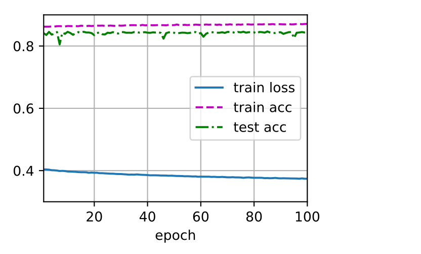
最后定义训练函数，采用随机梯度下降连续训练 100 次

def train(net, train_iter, test_iter, loss, num_epochs, updater):  
    animator = Animator(xlabel='epoch', xlim=[1, num_epochs], ylim=[0.3, 0.9],
                        legend=['train loss', 'train acc', 'test acc'])
    for epoch in range(num_epochs):
        train_metrics = train_epoch(net, train_iter, loss, updater)
        test_acc = evaluate_accuracy(net, test_iter)
        animator.add(epoch + 1, train_metrics + (test_acc,))
    animator.close()
    train_loss, train_acc = train_metrics
    assert train_loss < 0.5, train_loss
    assert train_acc <= 1 and train_acc > 0.7, train_acc
    assert test_acc <= 1 and test_acc > 0.7, test_acc

num_epochs = 100
lr = 0.1

def sgd(params, lr, batch_size):
    with torch.no_grad():
        for param in params:
            param -= lr * param.grad / batch_size
            param.grad.zero_()

def updater(batch_size):
    return sgd([W, b], lr, batch_size)

train_iter, test_iter = load_data_fashion_mnist(32, resize=64)
train(net, train_iter, test_iter, cross_entropy, num_epochs, updater)

显示的效果如下图，

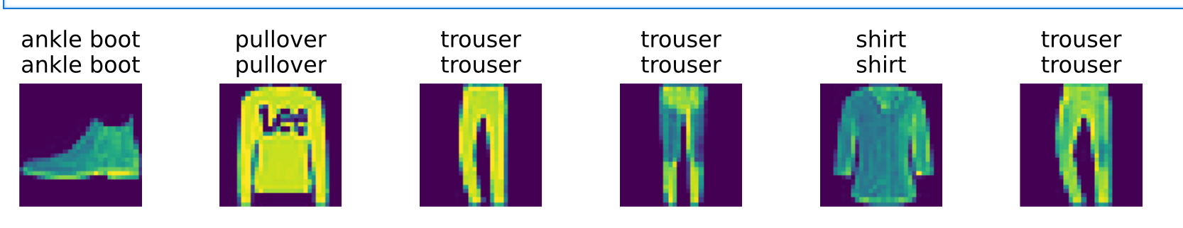
可以通过下面的预测函数查看训练的效果，因为每个 batch 是按照 32 的大小来读的，所以只需要拿出第一批迭代的数据，用这批数据的前六个来进行预测。

def get_fashion_mnist_labels(labels):  
    """返回Fashion-MNIST数据集的文本标签。"""
    text_labels = [
        't-shirt', 'trouser', 'pullover', 'dress', 'coat', 'sandal', 'shirt',
        'sneaker', 'bag', 'ankle boot']
    return [text_labels[int(i)] for i in labels]

def predict(net, test_iter, n=6):  
    for X, y in test_iter:
        break
    trues = get_fashion_mnist_labels(y)
    preds = get_fashion_mnist_labels(net(X).argmax(axis=1))
    titles = [true + '\n' + pred for true, pred in zip(trues, preds)]
    show_images(X[0:n].reshape((n, 28, 28)), 1, n, titles=titles[0:n])

predict(net, test_iter)

从下图中可以看到预测的结果和实际结果都是一致的。

Softmax的简洁实现 #

下面主要根据 pytorch 中已有的库来简化线性回归的实现。首先调用框架中现有的API来读取数据，只需要导入 data 的库

net = nn.Sequential(nn.Flatten(), nn.Linear(784, 10))

def init_weights(m):
    if type(m) == nn.Linear:
        nn.init.normal_(m.weight, std=0.01)

net.apply(init_weights);

loss = nn.CrossEntropyLoss()
trainer = torch.optim.SGD(net.parameters(), lr=0.1)

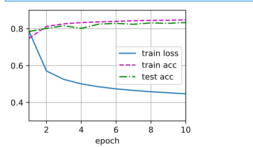
num_epochs = 10
train(net, train_iter, test_iter, loss, num_epochs, trainer)

执行结果如下，

Last modified on 2025-07-19